How to Design a Calibration Target for Your Specific Application

Accurate imaging systems play an important role in the modern world, ensuring precision in industrial applications, or allowing virtual objects to be superimposed in augmented reality. The foundation of these systems is calibration, a process that corrects imperfections such as lens distortion and sensor misalignment allowing us to measure the size of an object in world units, or determine the location of a robot all based on the images taken by a camera.

Effective calibration depends on many factors which is why selecting the right calibration target is crucial. Without it, even the most advanced cameras produce unreliable data, leading to errors such as misaligned 3D maps or robot localization failures. The calibration target design must be directly influenced by the camera system's field of view and constrained by practical factors such as working distance and manufacturing quality.

To establish a framework for calibration target design and selection, we’ll begin by explaining the relation between focal length and field of view, which establishes the optical limits of the system and lays the groundwork for understanding how working distance then dictates target size.

How Focal Length and Sensor Size determine the Field of View

Focal length is the distance between the focal plane (the plane of the camera sensor) and a reference point within the lens, known as the nodal point, when the lens is focused at infinity.

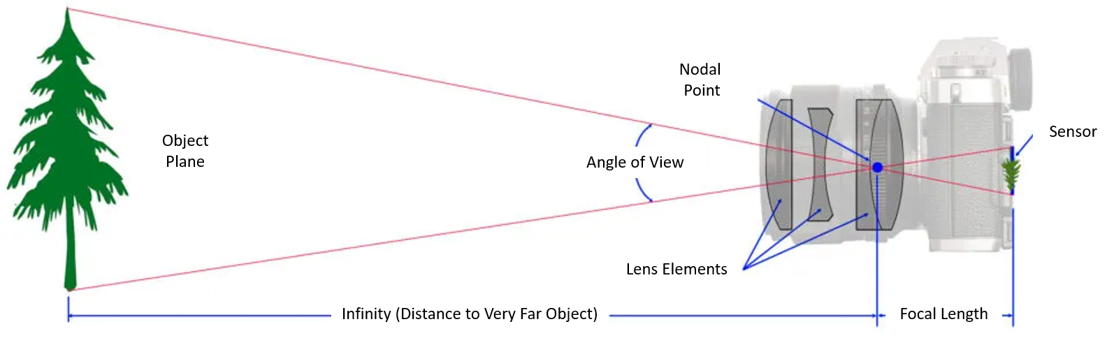
Focal length is an intrinsic property of the lens, determined by its optical design and directly influences the Field of View (FOV). However, the FOV also depends on the camera’s sensor size, which is the physical area of the image sensor. When paired with the same focal length lens, larger sensors provide a wider field of view compared to smaller sensors. This difference is sometimes described using the crop factor, which is the ratio of a full-frame sensor size to the sensor size of a given camera.

Visualization of the approximate angle of view of lenses with different focal lengths

The Field of View is the viewable area captured by an optical system. It can be expressed as a linear dimension (mm) or, more commonly, as an angular measurement (degrees) or angle of view.

Note: The horizontal FOV is used for convenience, but it's crucial to consider the sensor's aspect ratio (the ratio of its width to its height). This ratio determines the vertical FoV, ensuring that the entire target fits within the image frame.

To calculate the angle of view, we can use the pinhole camera model:

The tool below can be used to simplify the calculations:

How to Calculate the Proper Calibration Target Size for Your Field of View

Because the field of view (FOV) defines the captured scene's physical extent, the design of a calibration target is fundamentally influenced by the lens's focal length, the camera's sensor size, and the application's working distance.

We can calculate the optimal target size, knowing that the target must be large enough to cover a significant portion of the camera's angle of view at a given working distance.

Target Size =FOV * Coverage Percentage = 2 * WD * tan(AOV/2) * Coverage %

To ensure optimal calibration, the target should fill a considerable part of the camera's FOV, ideally 50-70%, when the target is positioned parallel to and facing the camera at the intended working distance. This provides enough features for accurate parameter estimation.

Note: For optimal results, calibration should be performed with the camera focused at the application's working distance. It is also crucial to maintain this focus setting throughout and after the calibration because changing the focus settings will alter the lens principal distance invalidating the estimation of the camera parameters.

Features and Feature Resolution

A feature refers to a distinct, detectable point or pattern element on the calibration target, such as the intersection points of a checkerboard, the circle centers of dot grids, the marker corners, and unique IDs of ArUco and AprilTags. It's a specific visual marker that the calibration software can identify and locate within the image.

In a checkerboard, the feature that calibration software detects is the corner point where four squares meet. In an ApriTag, features are the marker corners and unique ID.

Feature resolution is how accurately the calibration software can locate target features. It is measured in pixels, and pixel-level accuracy means within a pixel. However, advanced algorithms allow for sub-pixel accuracy, for example, tools such as OpenCV and MATLAB, can measure in fractions of a pixel, which is crucial for high-accuracy calibration.

A small calibration target, compared to the field of view, may result in insufficient feature resolution, limiting the software's ability to identify pattern elements. On the other hand, a target that’s too big could lead to practical issues, such as possible flatness problems or uneven illumination. The goal is to select a calibration target that is large enough to provide sufficient features while still being practical for the application.

How to Choose The Calibration Pattern Type?

Calibration relies on accurate pattern detection to estimate the intrinsic and extrinsic parameters of the camera. The most common types of patterns are checkerboards, dot grids, and coded markers like ArUco and AprilTags, each of which offers unique advantages and disadvantages. To choose a suitable pattern for your application it is helpful to consider the following:

Ease of Use
- Checkerboard targets are the simplest to implement and analyze, requiring minimal setup and processing.
- Coded patterns and dot patterns may require more complex generation and detection methods.
Environment
- Coded patterns like AprilGrids and ChArUco Boards are ideal for environments with variable lighting and potential occlusions, offering robust detection in dynamic settings.
- In controlled environments such as a laboratory, a chessboard may be sufficient.

Accuracy
- Dot or circle patterns are ideal for high-precision applications like metrology, as they allow subpixel localization of features. They also excel at calibrating imaging systems with distortion making them suitable for systems with a wide FOV.

How to Select a Suitable Pattern Density?

Pattern density refers to how closely packed the features are on the target. If the camera sensor has a high resolution it can detect smaller features. However, if the pattern is too close together, the sensor might not be able to distinguish individual features.

The goal is to ensure each square or marker is big enough to avoid blurry edges (black-to-white transitions) but small enough to fit multiple squares resulting in more data points which improves calibration accuracy.

To link pattern size to camera resolution, we can start by considering the smallest feature detectable on the image sensor:

Feature Size (image) = Pixel Size × Pixels per Feature

where:

Pixel Size = Sensor Size / Image Size= Sensor Width / Horizontal Resolution

This is the minimum detectable size of an object when viewed through a camera. However, to find the minimum resolvable size of the real-world object we must take into account the system’s magnification:

m = Image Size / Object Size= Sensor Width / Horizontal FOV Feature Size (object) =Feature Size (image)m

feature size (object) = feature size (image) / m

Note: Horizontal measurements are used for convenience, but we will generalize this expression later.

Combining these factors we can estimate a minimum feature size:

Feature Size (object) = Sensor Width / Horizontal Resolution × Pixels per Feature × Horizontal FOV / Sensor Width

The same principles apply to vertical measurements, so we can generalize the formula:

Feature Size (object) = FOV / Resolution × Pixels per Feature

It is worth noting that this calculation is not for the size of the square but for the minimum edge transition that the camera can resolve. A practical guide is that the pixels per feature should be at least 5 to prevent aliasing by providing a smoother gradient field for accurate subpixel fitting. To link this to pattern density we should use a scaling factor to calculate a square size that is large enough to accommodate the edge transitions and provide sufficient spacing between features.

These calculations provide a theoretical minimum to ensure sufficient resolution for calibration. However, it is also important to consider practical factors such as printing tolerances and the specifications of the calibration software used.

Manufacturing tolerance: It is essential to balance the pattern density with the ability to manufacture the target accurately. If the theoretically calculated feature size is too small to be manufactured with precision, it will be necessary to increase it to a size that matches the capabilities of the printing process. As a rule of thumb, the minimum feature size should be at least 2 times the manufacturing tolerance.
Lens Distortion/Blur: It's also important to remember that lens distortion can alter feature sizes within the image, potentially impacting overall accuracy. Therefore, allocating extra pixels per feature is considered a good practice
Feature Spacing: While the size of the markers is important, their spacing is just as relevant. Adequate separation between markers is necessary to ensure reliable calibration results.

For most applications, extreme precision isn't necessary. This allows us to design a reliable calibration target based on practical use cases as long as we follow some general rules such as:

Odd-even rule: To avoid rotational ambiguity, either rows or columns must have an odd number while the other must have an even number. If both rows and columns are even, the board becomes rotation-invariant, which can confuse detection algorithms.
White Border: A white border (10–20% of total board size) creates a high-contrast boundary that isolates the pattern, helping algorithms distinguish the pattern from the background.

Tools and Software for Pattern Generation

Online Camera Calibration Pattern Generator: This tool allows creating custom calibration patterns, such as checkerboards and AprilGrids with adjustable parameters like the number of rows and columns, tag size, and spacing.
OpenCV: Open-source library that provides functions for generating various calibration patterns, such as circle grids and ChArUco boards, in addition to its robust camera calibration and feature detection capabilities.
MATLAB: Powerful and flexible environment for generating and customizing calibration patterns, particularly through its Computer Vision Toolbox, which includes example patterns for natively supported calibration types. It also excels in advanced calibration tasks like distortion modeling and error minimization.

Material Selection

The material used for the calibration target is important for several reasons, including its impact on durability, flatness, and overall performance. Some commonly used materials are:

Paper or Vinyl: These are cost-effective, easy to print on, and replaceable, making them ideal for initial testing and prototyping. However, they lack durability and flatness for high-precision applications.
Aluminum Composite: ACM can be machined to create a surface free from imperfections, it also offers durability and its rigidity helps maintain flatness, making it suitable for industrial settings.
Polyurethane: Offers a good balance of durability and flexibility, and can be used in a wide range of applications. It is also very resistant to chemicals.
Glass: Provides superior stability, flatness, and low thermal expansion making it suitable for applications requiring high precision, such as microscopy and metrology.

Considerations

Finish: A matte finish is generally preferred to minimize reflections.
High contrast: Calibration algorithms rely on identifying distinct features so a high contrast between the pattern and the background makes these features easier to detect.

Conclusion

Designing an optimal calibration target requires matching your camera’s specifications and the application’s demands (FOV, working distance, environmental conditions) to the target size, pattern type, and density. By carefully considering these factors, you can create or select a calibration board that optimizes your camera system's reliability ensuring accurate calibration.

Nevertheless, the precision of any calibration setup is substantially limited by the quality of the target itself as imperfections like non-regular aspect ratios or low-quality prints introduce significant errors. This is why maintaining high contrast, perfect flatness, minimal manufacturing tolerances, and using non-reflective materials is crucial. To ensure these quality standards are met, it's often best to work with a specialized printing service that understands the unique requirements of calibration targets. Foamcoreprint uses industrial-grade materials and high-resolution printing techniques to minimize tolerances ensuring your target meets the demands of your application.

Resources